random html 4

Title Why Estimate Pollens by Zip Code? And How Might This be Accomplished?
Author(s) Este Geraghty, MD, MS, MPH American River College, Geography 350: Data Acquisition in GIS; Spring 2008 Contact Information: 4150 V Street, PSSB 2400 Sacramento, CA 95817 (916)734-5265 email: emgeraghty@ucdavis.edu Intern: David Soule
Abstract Pollens play an important role in human respiratory irritation. Many individuals require emergency level care when pollen levels are high and symptoms become intense. In any study of environmental health effects for which respiratory problems are considered, major ambient confounders must be dealt with. This paper describes such a project, justifies the need for a pollen estimation algorithm, and suggests data sources and a model for accomplishing such an estimation.
Introduction Pesticides, as a part of integrated vector management systems can cause health problems¹. In order for public health pesticides to provide more benefit than harm, they must be efficacious, inexpensive, and they must not pose unreasonable health risk². In the United States, safety issues surrounding the widespread use of public health pesticides have come to the forefront with the emergence of WNV. Since its arrival in the United States in 1999, 23,998 cases of human WNV infection have been reported, including 9,857 individuals with neuroinvasive disease and 963 fatalities³. Methods used in this country to prevent human infection range from avoiding mosquito bites and larvaciding (killing juvenile mosquitoes) to the more controversial adulticiding measures. The pyrethrin pesticides used for adulticiding have known human health effects, leaving health officials to contemplate the risk-to-benefit ratio in their efforts to prevent devastating WNV infections by using potentially toxic pesticide spraying applications. In order to accurately characterize risk from pyrethrin pesticides, rigorous research is needed¹. Unfortunately, at this time, little is known about the human health response to aerially sprayed pyrethrin pesticides that might guide policy makers in their safety assessment for this methodology. This may stem partly from the fact that environmental studies are made difficult because of confounding by environmental factors and the generally small effect sizes. The purpose of my overarching research project is to examine the safety of aerial spraying of pyrethrin pesticides for WNV mosquito control with regard to acute respiratory, neurologic, skin and eye complaints while adjusting for other relevant environmental exposures. As a small but important component of the project, I will begin the analysis of environmental factors, specifically tree, weed and grass pollens in relation to the study of respiratory illness, both because they are confounders/effect modifiers, and because the assessment of human exposure to these factors is often poorly measured.
Background Various pollens and mold spores have been found to be associated with acute respiratory irritation. In 1981, a study by Klabuschnigg, et al. showed a relationship between pollen/mold spore levels and childhood asthma attacks⁴. More recently, a 2006 report by Murray, et al. also indicated that pollen exposure was correlated with hospitalization for asthma exacerbation in children⁵. A study by Targonski found that asthma mortality in children (from age 5) and young adults (to age 34) in Chicago was associated with elevated mold spore levels⁶. And the literature has many additional examples of the effects of ‘aerobiology’ (organic particles) on respiratory problems. So in order to account for these essentially ‘allergy-related’ respiratory problems (especially asthma exacerbations) as relevant confounders and/or effect modifiers, it will be important to describe and quantify pollen and mold spore levels. Environmental health studies employing geographic information systems (GIS) constitute a growing field. However, for many environmental exposures, effect sizes are small⁷, requiring large datasets for adequate power to detect differences. Ideally, individual subject addresses at the point of exposure would be used to obtain coordinate (latitude and longitude) information in such studies. But personal address information is considered Protected Health Information under the Health Insurance Portability and Accountability Act (HIPAA) Privacy Rule and would therefore be subject to informed consent⁸. Such an undertaking is neither practical nor feasible for most researchers. Large human health datasets are available for research purposes that would be useful in environmental exposure studies. In California, for example, the Office of Statewide Health Planning and Development (OSHPD), collects millions of data records annually on emergency room visits and hospital inpatient discharges⁹. Patient-level geographic data is provided as the 5-digit zip code of residence. According to HIPAA, with a data use agreement, the 5-digit zip code can be considered ‘de-identified’ data and may be used without obtaining each individual’s informed consent¹⁰. So in order to take advantage of the large amounts of health information available in these databases, determination of environmental exposures at the level of the 5-digit zip code will be useful. Most of the studies found in the medical literature that estimate environmental variables at the zip code level use spatial interpolation techniques, that is, the prediction of variables at unmeasured locations is based on a sampling of the same variables at known locations¹¹. Inverse distance squared weighting, a method whereby data from a pre-specified number of nearest monitoring stations to the location of interest are weighted against the inverse of the Euclidian distance squared, is perhaps the most common interpolation technique used. More advanced spatial epidemiologists may employ Kriging, a statistical technique based on a weighted-moving-average interpolation scheme in which the set of weights assigned to samples minimizes the estimation variance¹². But these simple interpolation methods by themselves are limited in cases where the zip code of interest has a higher level of the environmental variable than any of the nearest monitoring stations, because these methods can never interpolate a level higher than that of the nearest monitor’s highest levels. A further limitation related to pollen and mold spore estimation is the sparse number of monitoring stations nationally. Spatial prediction is a more powerful method for estimation of environmental variables. Spatial prediction differs from interpolation in that the estimates are based, at least in part, on other variables (eg. through regression)¹¹. For example, Hoek et al. used an estimation method that includes not only a pollution interpolation estimate but also added covariates for population density and nearness to major roadways in each location studied¹³. In the study of pollen and mold spore exposure, selection and analysis of appropriate covariates will be critical. According to Fumanal et al. ragweed pollen release is most dependent on plant density and plant biomass¹⁴. And in an email conversation with Dr. Fumanal, he notes that plant biomass is related to habitat including: soil quality, temperature, precipitation and elevation. Plant density, combining all pollen producing plants (trees, grasses and weeds) may be determined by evaluating landcover surface rasters, while soil maps, elevation maps and meteorologic data may be downloaded and used as a surrogate measures for plant biomass. Our pollen estimation model will include these data as covariates as well as seasonality for various pollen types and pollen counts obtained from monitors registered with the National Allergy Bureau. Because ‘gold standard’ validation techniques (measuring pollen levels directly against calculated estimates) are impractical for most researchers, statistical methods are frequently employed. Most often, researchers use jackknifing or bootstrapping (i.e. resampling techniques based on leaving out one observation from the original dataset to test the estimated parameter for that observation)¹⁵. Once estimations are made for pollens, we will use pollen monitoring station data for jackknifing validadtion (by monitoring station and year).
Methods Data Acquisition The different data types that will be used in the pollen estimation analysis will be discussed in detail below. Pollen Counts The National Allergy Bureau (NAB) maintains pollen monitoring stations across the United States and makes that freely data available upon request. Each pollen monitoring station must maintain quality standards as set forth by NAB. Two types of pollen monitors may be used: Burkhard or Rotorod. For each station, pollens are counted on a regular schedule (most are daily, but a few perform weekly counts only). Pollens are categorized by their specific type. The data is provided to researchers in the form of an Excel spreadsheet. Four years of pollen data (2003-2006) will be used as gold standard measures against which to relate our calculated estimates.
The pollen data will need to be reclassified to clinically relevant categories of “trees,” “weeds,” and “grasses.” Using the reclassified data, pollen seasons for each class and each monitor location can be determined. Each monitoring station will also need to be geocoded and mapped. The processing algorithm is shown at the right:
Vegetation Data The vegetation data was obtained from the following CDF Fire and Resource Assessment Program site, http://frap.cdf.ca.gov/data/frapgisdata/download.asp?rec=fveg02_2 The original dataset has a 100 meter resolution based on the 1866 Clarke Datum, projected into an Albers projection. The original dataset was based on wildlife habitat characteristics. We reclassified the map into the following categories: trees, herbaceous, shrubs, agriculture, urban, and none. Categories such as: barren/other, desert, water and wetland, were all reclassified to none (no data). Further, although trees represented a single category, there were also separate categories for conifer and hardwood. Since both of the latter tree types do produce pollens that may cause respiratory irritation, they were reclassified to be included in the “trees” category.
Reclassifications were performed using: Spatial Analyst Tools/Reclass/Reclassify tool. Then the reclassified raster data was vectorized using: Conversion Tools/From Raster/Raster to Polygon tool. There are 821,420 separate polygons in this data.
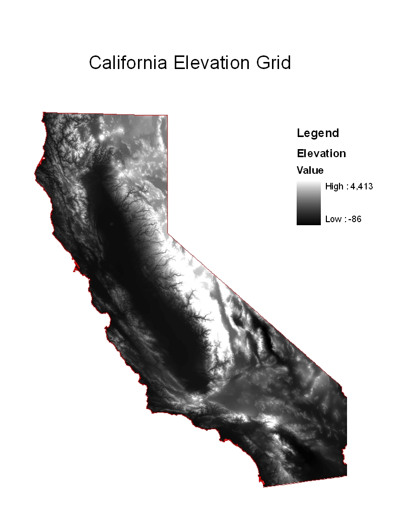
Soils Data Soils data was downloaded from STATSGO. The data is in tabular form with an accompanying map. Within the tables there are several fields that appear promising including: Vegetative productivity index, available water supply, range production, yields of non-irrigated crops, forest productivity, yields of irrigated crops, range production. We will contact the Natural Resources Conservation Service (NRCS) and/or UC Davis agriculture department to help us determine which variable(s) best suit our need for pollen habitat suitability. Climate Data Climate data were obtained for 4 years (2003-2006) from the California Air Resources Board. Data are measured hourly for over 300 monitoring stations in the state. The data include temperature, precipitation, wind speed and direction (see below) and other data points. Temperature and precipitation data will need to be summarized into daily min, mean and max for use in the model, pertaining to habitat suitability. For each variable, a surface will be created using either a spline function or simple kriging. The surface will then be vectorized and re-aggregated to the zip code level (centroids) for averages. Zip Codes Zip code maps for years 2003-2006 were obtained from the Centers for Disease Control and Prevention GIS library. The zip code maps are to represent the level at which pollens are calculated in the state of California. This was chosen because future analyses will include human subject data that are geocoded to the patient’s residential zip code. Wind Speed and Direction Pollen monitors detect the pollens that they ‘see.’ But this does not necessarily mean that those pollen originated from that very location. In fact, the monitor is detecting pollens that have been dispersed to that location from somewhere else. This is why we must account for wind speed and direction in our model. Although we can calculate where pollens are produced, we must determine where they will go from there. To do this we will use a simple wind rose. Here is how it works: Say you have a data point on a day that the wind is 15 mph and 225degrees. You can construct a wind rose that indicates the direction that the wind is coming from (225degrees means wind from the SW-erly direction). To find the x coordinate, one must multiply 15 x cos (225degrees). The y coordinate is found by multiplying 15 x sin(225degrees). This will give you a vector of the wind velocity for that point in time. Elevation Data The elevation raster is a product of: 1) multiple downloads from the National Elevation Dataset, 2) the mosaic to raster operation (including projection), and 3) an extraction based on a mask. The National Elevation Data Set can be obtained from http://ned.usgs.gov/ with subsequent links to the National Map Seamless Viewer http://seamless.usgs.gov/, the location from which the actual data is requested. Some 55 separate downloads of 1 arc second data were required to secure all the data for the state of California. Some downloads proved to be corrupted, or incomplete. Ultimately, approximately 50 separate tiles were used for the mosaic operation. The mosaic operation was completed in a multi-step process which first required the unzipping and review of each separate tile to insure that the entire state was covered by elevation data. Gaps were filled using later downloads. Tiles were then chosen based on their location and then stitched together in three separate operations to create first an outline (essentially the border of California), and then two interior mosaics, one for the interior north and one for the interior south. This was performed using the model “Mosaic to New Raster” in Data Management Tools/Raster. This model also allows for the projection of rasters (I chose to project them to match the mask -- NAD 83 California (Teale) Albers available as a Projected/State System. It also allows for the choice of Mosaic Method – (our choice was “mean”). This was done for each of the preliminary mosaics as mentioned above and then again to assemble them together to make the final statewide raster. We chose to do this in a multi-step process because we found that as we placed more rasters on the map (before any mosaic operation), the redraw rate became untenable. As a measure of computer processing burden this kind of work entails, the four mosaic/projection operations required a total of 8 hours and 29 minutes.
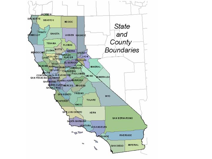
The downloaded data included data beyond the borders of California. To clip away that data we constructed a mask. We used the US Forest Service Pacific Southwest Region GIS Clearinghouse Site to download the State And County Boundaries (http://www.fs.fed.us/r5/rsl/clearinghouse/gis-download.shtml). This data includes a very detailed California boundary, including all offshore islands, such as The Farallones, the Channel Islands, and other “rocks”. It also includes neighboring counties of Nevada and of Oregon. This is a feature class with some 168 records, i.e. 168 separate polygons. It was sourced from a 1:24,000 scale map and has an estimated margin of error of +/- 7 meters. It is in the NAD 1983 Albers projected coordinate system which is an Albers Conical Equal Area projection. The Geographic Coordinate System is GCS_North_American_1983. The horizontal datum is NAD 83, and the ellipsoid is GRS 80. The measurements are metric.
To create the final mask for elevation raster extraction we used the State and County Boundaries feature class and ultimately excluded the Nevada, and Oregon counties and the smaller offshore islands. The resultant data for the California elevation map are as follows: -Size: 4.67 GB uncompressed. -Cell Size; 27.718 x 27.718 -It is an Esri Grid, with 32 bit floating point, projected to NAD 83 Albers -Unit of measurement is meters This elevation map will require further processing. The most likely next step is to determine if there are elevation categories related to: 1) habitat suitability for pollen producing plants and 2) barriers for pollen dispersion.
Results The main study question for this project was “How might one accomplish pollen estimation by zip code?” The methodology section above outlines how free data sources might be processed for use in an estimation model. It also shows several datasets that have been partially processed at this time. No further results related to estimating pollens are available.
Conclusions Few environmental health/respiratory health studies endeavor to use pollens in their models (as confounders or effect modifiers). This is probably because the process is quite difficult. Simple interpolation will not work since so few pollen monitors exist in the state (7 monitors). Therefore more complex models must be used. Still, since pollens do play a significant role in respiratory irritation that may lead to emergency care, they must be considered. This project review the data that would be necessary to create a model for pollen estimation by zip code. Zip codes are a relevant spatial class since they are the smallest area for which large human subject datasets can be aggregated (due to HIPAA regulations).
References 1. U.S. Environmental Protection Agency. Pesticides: Health and Safety. July 9, 2007; http://www.epa.gov/pesticides/health/human.htm. Accessed July 11, 2007. 2. World Health Organization. WHO Pesticides Evaluation Scheme: "WHOPES". 2007; http://www.who.int/whopes/en/. Accessed July 5, 2007. 3. Centers for Disease Control and Prevention. Statistics, Surveillance and Control. July 10, 2007; http://www.cdc.gov/ncidod/dvbid/westnile/surv&controlCaseCount07_detailed.htm. Accessed July 12, 2007. 4. Klabuschnigg A, Gotz M, Horak F, et al. Influence of aerobiology and weather on symptoms in children with asthma. Respiration. 1981;42(1):52-60. 5. Murray C, Poletti G, Kebadze T, et al. Study of modifiable risk factors for asthma exacerbations: virus infection and allergen exposure increase the risk of asthma hospital admissions in children. Thorax. December 29 2006;61(5):376-382. 6. Targonski P, Persky V, Ramekrishnan V. Effect of environmental molds on risk of death from asthma during the pollen season. J Allergy Clin Immunol. May 1995;95(5 pt 1):955-961. 7. Wellenius G, Schwartz J, Mittleman M. Particulate air pollution and hospital admissions for congestive heart failure in seven United States cities. Am J Cardiol. Feb 1 2006;97(3):404-408. 8. Office for Civil Rights - HIPAA. Medical Privacy - National Standards to Protect the Privacy of Personal Health Information. May 16, 2006; http://64.233.167.104/search?q=cache:B94RauCD2ekJ:www.hhs.gov/ocr/hipaa/privacy.html+protected+health+information&hl=en&ct=clnk&cd=9&gl=us. Accessed March 17, 2007. 9. Office of Statewide Health Planning and Development. Medical Information Reporting for California (MIRCal). January 23, 2007;http://www.oshpd.ca.gov/MIRCal/index.htm. Accessed March 17, 2007, 2007. 10. National Institutes of Health. How Can Covered Entities Use and Disclose Protected Health Information for Research and Comply with the Privacy Rule? Feb. 2, 1007; http://privacyruleandresearch.nih.gov/pr_08.asp. Accessed March 17, 2007. 11. Bolstad P. Chapter 12: Spatial estimation: interpolation, prediction and core area delineation. GIS Fundamentals: A first text on geographic information systems. Second Edition ed. White Bear Lake: Eider Press; 2006:395-433. 12. U.S. Environmental Protection Agency. Glossary of Geostatistical Terms. April 1991; http://www.sph.umich.edu/geomed/htmls/glossary/geoeas.glossary.html. Accessed July 13, 2007, 2007. 13. Hoek G, Fischer P, Van Den Brandt P, Goldbohm S, Brunekreef B. Estimation of long-term average exposure to outdoor air pollution for a cohort study on mortality. Journal of Exposure Analysis and Environmental Epidemiology. 2001;11(6):459-469. 14. Fumanal B, Chauvel B, Bretagnolle F. Estimation of Pollen and Seed Production of Common Ragweed in France. Ann Agric Environ Med 2007; 14:233-236. 15. Buishand TA, Beersma JJ. Statistical tests for comparison of daily variability in observed and simulated climates. Journal of Climate. October 1996 1996;9(10):2538-2550.